Hi guys,
I love database theory because it includes mathematics, statistics, logic, programming and data organization.
I wrote this post because i read a post on linkedin about the well known "201 bucket limitation" in the statistics used in SQL Server.
Bob Ward (the Principal Architect at Microsoft, in the photo on the right while dreaming statistics and rugby...lol ) rensponded to the author of the linkedin post asking him to give a real example where this was a limitation. He also said he would verify.
I then asked myself whether the logic with which statistics are managed could not be improved in any way without increasing their size.
In the post on Linkedin was also referred to a post of the well-known mr. brent Ozar: The 201 Buckets Problem, Part 1: Why You Still Don’t Get Accurate Estimates
Brent used the Stack Overflow 2010 database database for his examples and I will do the same in this post.
If you want to follow my examples then, first of all, download the Stack Overflow 2010 database.
This is the first post of the year so I WISH YOU AN HAPPY NEW YEAR 2023 to all the thousands of friends who follow me regularly.
More than 7500 friends...WOW!
I don’t know if I deserve it but it is really a pleasure for me.
Enjoy the reading ...
Indexes and Statistics
Statistics, in SQL Server, are very important objects because they are used to estimate cardinality. Proper cardinality is needed to produce the best execution plan possible.
For example if I know I have few data in a table when I perform the logic JOIN operator I could use the best physical operator: in this case a Nested loop operator.
If I had multiple lines I would have used different physical operators.
Now, when I add an index to a SQL table at the same time a statistic is created.
This object is one data page wide and therefore 8 Kb.
Yes, a single data page and no more than one. Within a data page I can enter a maximum of 201 buckets.
How Statistics are currently managed
Have you already downloaded, unzipped and attached the database we were talking about before?
Then go!
Open your SSMS and then, to generate a statistic, we will create a new index.
We will create an index on the users table by executing the following T-SQL command:
CREATE INDEX idx_Users_Location ON dbo.Users(Location);
Now we have a new statistic whoose name is the same of the index.
We can
show what this statistic contains using the DBCC Show_Statistics T-SQL command:
DBCC SHOW_STATISTICS ('dbo.Users', 'idx_Users_Location')
The output is divided in the sections:
The upper section is a sort of master table that contain information such an the name of the statistics, the number of rows of the table, the number of buckets used.
We have also the field Average Key length Average that represent then number of bytes per value for all of the key columns in the statistics object.
Finally, we have the Density field that is information about the number of duplicates
in a given column or combination of columns and it is calculated as
1/(number of distinct values). But it is not used by the query optimizer. It is displayed for backward compatibility with versions before SQL Server 2008.
In the middle section we have a summary of all the data in the table.
We have two rows.
Each row shows data related to the columns indicated in the columns field.
- The first row so shows data related to the column Location.
- The second row shows data related to the columns Location, Id.
The Value contained in the All density column is given by the formula 1 / distinct values.
(As said distinct values are related to the columns indicate in the column field)
The
Average length column represent a the number of bytes needed to store a list of the column values for the
column prefix.
The lower section contain data related to each bucket sampled.
Now, since the table Users has almost 300.000 rows our 201 buckets are all used.
The data in this table is very important, so we need to understand what the various columns mean.
The RANGE_ROWS column means that in the range of location between the previous bucket and the bucket we are reading there are N rows excluding the values indicated.
Taking a look at the row highlighed in the photo above, in the range of locations between
Adelaide (Australia) and Ahmadabad (India) there are 54 rows excluding
Adelaide and Ahmadabad.
The value of the EQ_ROWS column indicates how many rows there are in the bucket.
In the example, the bucket where the RANGE_HI_HEY is equal to the value "Ahmadabad" has an EQ_ROWS value of 159. This means that for the Ahmadabad position we have exactly 159 rows.
The next column DISTINCT_RANGE_ROWS indicates the distinct number of values.
The value 25 means that of the 54 rows of the RANGE_ROWS group there are 25 distinct locations.
Finally we have the AVG_RANGE_ROWS column. This value indicates the average number of rows between the previous bucket and the bucket we are watching.
In the example the value 2.16 means that if you search for a location between Adelaide and Ahmadabad, SQL Server estimate that there are 2.16 rows.
You can get this value by dividing 54 rows by 25 distinct value.
A simple consideration!
In case we search for a value present in the RANGE_HI_KEY column of a bucket we know a lot of information.
For example if we search for the location Ahmadabad we know that there are 159 rows (EQ_ROWS) with 25 distinct values (DISTINCT_RANGE_ROWS).
That's great!
If instead we search for a a value that is not present in the RANGE_HI_KEY column of a bucket we know less information.
We know only how many rows and the average number of rows there are between a bucket and the previous one. (RANGE_ROWS and AVERAGE_RANGE_ROW columns).
In this case estimate is less accurate!
Is less accurate principally beacuse we assume that the data is evenly distributed while in reality this is often not true at all.
Logically the number of rows does not depend by the logically order of the location.
We see this in this example.
As we seen from the statistics from location Adelaide to Ahmadabad...
Select location from Users Where Location > 'Adelaide, Australia' and location < 'Ahmadabad, India'
..we have exactly 54 rows:
Using the following T-SQL command we can see that...
Select location, count(location) From users Where location > 'Adelaide, Australia' and location < 'Ahmadabad, India' group by location order by location
...our 54 rows are are not evenly distribuited.
In fact, we have 16 users in Adelaide (south Australia, Australia) but only 1 in Adelanto, California:
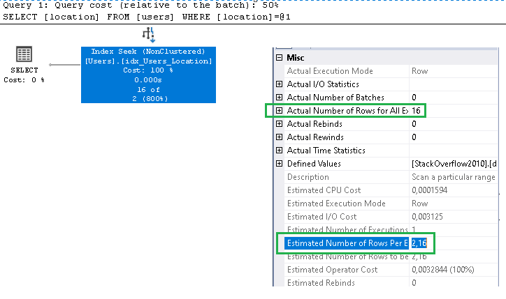
In each case SQL Server will use in the execution plan the value of 2.16 for the "estimates number of row".
Take a look to the following to cases.
1) Users from Adelaide, South australia, Australia
Select location From users Where location = 'Adelaide, South Australia, Australia'
We have 16 rows but the estimated number of rows is 2.16
2) User from Adelanto (CA)
Select location From users Where location = 'Adelanto (CA)'
We have 1 row but the estimated number of rows is always 2.16
The value used for the Estimated numer of Row parameter is not very precise.
SQL server use in the example the value 54 / 25 = 2.16 but i think it is not a very logical choice.
I mean that: the fact that from Adelaide (A) to Ahmadabad (B) i have 54 (N) rows tells me nothing about the number of rows a location within this alphabetical range from A to B may have.
The cardinality of a locality does not depend in any way on its name.
So logically a global value can be more rapresentative.
Yes, but what value can I use? ...what would be a good value?
Instead of the value 2.16 used by SQL Server, we can determine a more accurate value, by minimizing the value of the SUM(TOT) for the rows returned from the following SELECT in function of the parameter X.
Select COUNT(location) - X as TOT From users Group By location
For the data into the user table i get that the best value is equal to
10.615 and so a value five times great than the value (2.16) proposed by SQL Server.
What I propose to Microsoft!
My propose is to use a different value than the value read from the bucket (2.16)
I propose, if the data not evenly distributed beyond a certain threshold, we can use as the estimate number of rows a global value.
We can estimate if our data evently distribuited or not by evalutaing the standard deviation.
Then if the calculated value of the standard deviation is greater than a properly choosen threshold then we can use this new value.
What value we could use?
I propose to use this simple formula to get a value.
PROPOSED_VALUE = ( NUMBER_OF_ROWS - NUMBER_OF_NULLS_ROWS ) / ( NUMB_DISTINCT_VALUES -1 )
PROPOSED_VALUE = ( 299398.0 - 169193.0 ) / (12264 - 1) = 10.615
This value is the same value of the "teorical" value previously calculated.
As we seen previously, this value is more appropriate than value 2.16 because it "minimizes the sum of the differences".
Note that, I excluded all the rows where the location is null because this value have already a dedicated bucket in the statistics and also because it is very numerous.
Surely you should do many other tests on different data.
Probably i will do some more tests and I will tell you the results in a next post!
This is that a propose!
To conclude some reflection on the famous "201 bucket" limitation.
The 201 bucket limitation
As said previously, for each statistics we can have a maximum of 201 buckets.
A page 8 KB wide can not contain more than buckets.
Are 201 buckets few? .. or are they many?
Of course, there is no answer because it depends on the content of the table
If we have few data probably not all buckets may be used.
In this case, we will always read an 8 KB page of data.
Probably due to the fact that the size of the databases is constantly increasing, it might be profitable to dedicate more than one data page to statistics.
This statement must be evaluated but, It is true that it should be done not for all statistics but only when a single page is no longer enough.Otherwise we risk reading many more data pages with negative effects on performance.
Now the real question is: In what cases can the limitation of the number of buckets cause problems?
The "Miami example"
Take a look to this histogram.
In the RANGE_HI_KEY between Mexico and Michigan we have 288 row.
We have also 22 distinct values.
The AVG_RANGE_ROWS is therefore equal to 288 / 22 = 10,36.
Between data within this range there is the city of Miami which has well 99 users.
Miami has many users but not enough to have its own bucket in the statistics.
What's happens in this case?
Just take a look to the following case..
yes, if we search users located in Miami SQL server estimates 10 Rows, while actually the rows are 10 times as much.
There is really a big difference!
To conclude, if we have enough data to use all 201 buckets some problems can happen when we are dealing with data that recurs with a certain frequency but not such as to be put in a bucket.
Thanks you! That's all for today!
I hope you found this post useful!
~ Luke
Previous post: Temporal features and temporal tables clearly explained and with examples! (Special: WHO'S WHO in the SQL world pt/2.. Mr. Krishna Kulkarni)


Comments
Post a Comment