Cardinality in Multicolumn Statistics Vs. Compatibility level ...formulas, calculations and examples!

Hi guys,

Welcome to this post!

 

We all knows how much statistics are of vital importance for the performances.
If SQL Server estimates an incorrect cardinality it will also generate a non-optimal execution plan.

For example, we might find a join type not suitable for the number of lines to manage.

Used a nested loop join to read a table with millions of rows is like going from one side of the US to the other using a bicycle.
I am sure It will take a long time!

But the opposite can also happen...

If we used a join operator suitable to handle many lines when instead we have few would be like going to find the neighbour by plane. We would use a lot of resources unnecessarily.

Today we focus in the case of multicolumn statistics, let’s see how they are calculated and how this calculation has changed during the SQL Server versions and then at the change of compatibility level.

I remember we have just talked about this topic here: SQL Server, A little about composite indices and a little about the relative statistics ..

Enjoy!

 

 

Why statistics are important!

As we said earlier statistics are very important.

Statistics are objects inside the database that allow to calculate the cardinality (that is the number of lines) during the steps of the execution of a Query.
As we said, they are used to create a correct execution plan.

Let’s take a small example

Suppose you have a table called OrdRig that contains for example the rows of a sales order.

We have used this table in many other posts.

Our table will have a field pointing to a table that contains the list of products (productid) and there will then be a field for the Quantity and a field for the price.

Suppose you want to see all rows of a certain item and price.

We will write a Query similar to this:

 

SELECT * FROM ORDRIG WHERE [IDPRODUCTS]=2 AND [PRICE]=4
      

Statistics are used to estimate,even before the query is executed and when building the execution plan, how many lines will return our query.

 

And indeed they do!

If we look at the figure below we see that the table has 500 rows and that the Estimated Number of Rows is equal to 2.53 rows

The more precise this value is, the more we will have an optimal execution plan!

To berrer understand.

 

Suppose now to join with our ORDRIG table on a table that contains the list of products we call ITEM

 

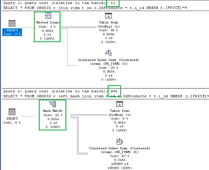
SELECT * FROM ORDRIG R JOIN ITEM T ON R.IDPRODUCT = I.ID WHERE R.[PRICE]=4
      

From the execution plan we can see that a nested loop operator is used to perform the join operation.

 

This happens because, thanks to the statistics, SQL server can estimate that a few rows will be returned from the ORDRIG table.

 

For example, a less accurate estimate of cardinality would have led SQL Server to opt for another less suitable join operator.

From the following picture we can see that if use the Hash Match operator to perform the join operation and instead of the nested loop operator execution time will be much much much worse (in this example the execution time is about 100 times greater)

Calculating cardinality is not an easy task when dealing with multiple columns!

...also because we can not store (and then also update) the frequency of all possible combinations

We will not talk today about how statistics work, this paragraph is just to highlight their importance.
Instead, we will see how the cardinality is calculated in the case of multicolumn statistics.

...but first let’s see how our test table OrdRig is made ...in case you want to repeat the same test!

The Table OrdRig

Use the following commmand to create the table OrdRig used in the tests

CREATE TABLE ORDRIG
(
[ID] [int] NOT NULL IDENTITY(1, 1),
[IDORDTES] [int] NOT NULL,
[IdProducts] [int] NOT NULL,
[Price] [float] NOT NULL,
) ON [PRIMARY]

Then use the following command to populate the table:

with u as (
    select 1 as n
    union all
    select n + 1
    from u
    where n < 500
)
Insert into OrdRig (idOrdTes,IdProducts,Price)
select
    1+ row_number() over (order by n) / 5,
       1+ row_number() over (order by n) / 11,
       1+ row_number() over (order by n) / 3
from u
option(maxrecursion 0);

Our table will have exactly 500 rows:

Now we define two statistics. 

 

A first statistics is defined on the two fields IdProducts and Price

create statistics I_IdProducts_Price on Ordrig(IdProducts,Price) with fullscan
      

We can show the content of this statistics using the command:

dbcc show_statistics(OrdRig,I_IdProducts_Price)
      

Some important information are showed:

The number of row of the table (500)
The number of row sampled (500)

A value called All density that in the examples that we will do is equal to 0.005076172

Another value read from the statistics that will be used in the following calculations is the value read from the EQ_ROW columns.

This value represents the number of rows within the range of values specified in the RANGE_HI_KEY column. Note that if a table has many distinct values the statistics do not contain every single value but data a grouped into a range of values.

 

 

A second statistics in defined only on the price field

create statistics I_Price on Ordrig(Price) with fullscan
      

These are the same properties for the second statistic.

 

Now we finally move to the calculation of cardinality in the case of multicolumn statistics!

We will see how the cardinality calculation changes based on the compatibility level.

 

Cardinality in multicolumn statistics Vs. compatibility level 

 

Calculation of cardinality with CL >= 14

The formula of the selectivity of the combined multi single-columns statistics is:

MAX( MIN( 'all density',p0,p1,p2,p3),  p0*p1*p2*p3)
      

With the following note:

• The term “All density” in the formula indicates the value of the column “all density” for the statistics that include both fields used in the clause WHERE (idProducts and price)

• The Terms p0,p1,p2,p3 are the selectivity value of each column used in the clause WHERE cwhere p0<p1<p2<p3
  

• If a multi-columns statistic has more than 4 columns, only the first 4 are used. The others are not used.

The calculation is as follows:


The ALL_DENSITY values, taken from the I_IdProducts_Price statistic, is 0.005076142

 

The selectivity p0 is the selectivity of the field IdProducts. 

 

Its value is equal to 11/500
Where the value 11 is read from the statistic in which the first column is IdProducts. 

In the query the value of Idproducts = 2 is in the range from 2 to 3 and its value is 11

 

p1 is the selectivity of the field price and its value, read from the statistic I_Price, is 3/500

For the sake of truth the two values of p0 and p1 should be exchanged because p0 is greater than p1 but the result of the calculations does not change in this case...

 

Now we have that the selectivity of the combined multi single-columns statistics is:

MAX( MIN('all density',p0,p1,p2,p3), p0*p1*p2*p3) =
 
MAX( MIN(0.005076142, 11/500, 3/500), 11/500 * 3/500) =
 
MAX( 0.005076142, 0.022000 * 0.006000) = 0.005076142

Finally the total cardinality is 0.00576142 * 500 = 2.53 

As shown in the following picture:

Calculation of cardinality with CL = 13

 

Under this CL we have the following formula:

MIN( 'all density', p0, p1, p2, p3) 
      

This time the value of the selectivity is:

MIN( 0.005076142, 11/500, 3/500) = 0.005076142
      

Selectivity of the combined multi single-columns statistics is 0.005076142 * 500 = 2.53

In this case we have the same result of the CL 14

Calculation of cardinality with CL = 12

 

Under this CL we have the following formula for the cardinality

p0 * p1^(1/2)
      

This time the value of the cardinality is:

11/500 * (3/500)^(1/2) = 0.022 * 0.077459 * 500 = 0,85 rounded to 1
      

 

Conclusion

We can see how in every new version of SQL Server the formula for the calculation of cardinality on the case of a multi-colored statistic becomes increasingly complex.
This is usually done to produce a more accurate estimate of cardinality.

 

That's all for today!! Have a nice week end!!

Luca

 

 

 

 

 

 

 

 

 

 

 

 

 

 

 

Previous  post:Azure Data Studio News! Now shows the execution plan!